Rating fluctuations in chess

2024-04-09

Exploring the ELO rating system and how ratings go up and down.

Tags: data probability chess

The ELO rating system, devised by physicist Arpad Elo, is used in chess to rank people by their playing ability. This post is an investigation into what a typical rating fluctuation looks like, an idea that probably came to me after a particularly devastating drop in my rating. But first, let's briefly review the ELO system.

The ELO system

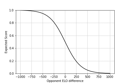
Let's say someone scores 1 point for winning a game, 0 points for losing a game, and 1/2 a point for drawing a game. If their ELO rating is $r_{A}$ and their opponent's rating is $r_{B}$, then their expected score (i.e. their average score over millions and millions of games) is, according to the ELO system,

$$\sigma(r_{A}, r_{B}) = \frac{1}{1+10^{(r_{B}-r_{A})/400}}.$$

This is a form of the sigmoid function, which is basically a fancy way of mapping numbers to the 0-1 range. It gives fairly intuitive results if we plug ratings into it. When $r_{A} = r_{B}$, the expected score is 0.5. Makes sense: equally strong players should win equally often. Beyond that, for every difference of 400 points between your rating and your opponent's, your expected score increases or decreases by about a factor of 10. If you're rated 400 points below someone, your expected score is about 1/10. 800 points below and it's about 1/100.

Note that this doesn't give us win, draw and loss probabilities. An expected score of 9/10 could mean a 0% chance of drawing and a 90% chance of winning, or it could mean an 80% chance of winning and a 20% chance of drawing. Among its other limitations, it also doesn't account for the advantage of playing the first move. The Glicko rating system tries to improve on the ELO system, but still ends up using the sigmoid function. Lichess, the best chess website ever, uses Glicko-2.

Here's a plot of ELO rating difference versus the expected score. If you're lagging behind someone by 800 points, you have a negligible chance of scoring anything against them. If it's only 100 points, however, then your scoring chances are actually decent, which makes me feel better for losing so many games to supposedly weaker players.

The last detail is how to update the ratings after a game. The player of rating $r_{A}$ is given a new rating of

$$r_{A} + K(s-\sigma(r_{A}, r_{B})),$$

where $s \in \{0,1/2,1\}$ is their score and $K > 0$ is the so-called "K-factor" that determines how quickly ratings change. The more your actual score differs from the expected score, the more dramatic the change in rating. So if you lose to a much worse player, $s-\sigma(r_{A},r_{B})$ will be negative and relatively large, and your rating will suffer a big drop of up to $K$ points. If you lose to Magnus Carlson, well, that was expected, and your rating will barely move. If you draw with someone of the same rating, then your rating won't change at all. None of this will be news to chess players.

What's a typical rating fluctuation?

ELO ratings are estimates of someone's "true" playing strength, assuming that such a thing exists and that it can be quantified as a single number. We'll consider two approaches to determining what a typical rating fluctuation looks like. The first approach is to simulate a bunch of games. The second is to model the rating and its fluctuations as a Markov process.

Approach 1: Simulation

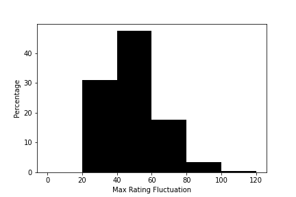
I ran 10,000 simulations of 100 chess games. The player is given an initial rating of 1800. This is their "true" rating, which remains fixed, but their rating for matchmaking purposes is updated after each game and they're matched against an opponent of the exact same rating. A K-factor of $K=10$ was used for the update formula, resulting in a rating change of +-5 points after each game, which seems to be about the standard for chess websites. Draws were disallowed, which meant that the probability of a win could be derived from the expected score: $P(\text{win}) = \sigma(1800,r)$, where $r$ is the player's current rating and thus the rating of their opponent.

Here's the distribution of rating fluctuations over all the simulations. It shows the maximum distance the player got from their original rating in each simulation. We see that it's highly unlikely to stay within 0-20 points of your original rating over 100 games. Most players will stray by 20-80 points. Of course, this is highly dependent on the number of games and the K-factor: more games and a higher K-factor will result in greater fluctuations.

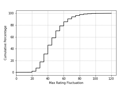
Here's the same thing as a cumulative distribution. As we increase the max rating fluctuation along the x-axis, the y-axis tells us the percentage of simulations that had a fluctuation less than that amount. We can see that ~80% of the time, the player stayed within 60 points of their original / true rating.

The moral of the story is that, even assuming that someone is a probabilistic machine who plays perfectly consistently and is never tired or tilted, they're still going to see significant variance in their rating. But still, if you keep blundering your pieces and lose 10 games in a row... it may be time to take a break.

Approach 2: Markov model

The distribution of rating fluctuation can also be computed by modeling the games as a Markov process, which I discussed previously in the context of board games. This saves us from running a bunch of simulations, and gives exact results rather than estimates.

Each possible rating is represented by a state in the Markov model. Let's say we're in the state $i$, corresponding to a rating of $r_{A}$. At each step of the Markov process, we increase or decrease our rating by 5 points (for $K=10$, as above), which sends us to the state corresponding to $r_{A}+5$ (label it $i+1$) or $r_{A}-5$ (label it $i-1$). If the transition matrix is denoted by $P$, then $P_{i-1,i} = \sigma(1800,r_{A})$, $P_{i+1,i} = 1-P_{i-1,i}$, and, for all other indices $j$, $P_{j,i} = 0$.

The vector $x^{(k)}$ gives the probability of being at each possible rating after $k$ games have been played. With probability 1, we start off at a particular state $i$. So $x^{(0)}_i = 1$ and $x^{(0)}_j=0$ for $j \ne i$.

I'm being vague about how many possible states there are, because that depends on how many games are played. For $N$ games, there are $2N+1$ states: we can win all $N$ games, lose all $N$ games, or anything in between. That results in $P$ being a $(2N+1)\times(2N+1)$ matrix, with its rows corresponding to the new rating after a game and its columns corresponding to the rating before the game.

To get the probability distribution of what rating we're at after $N=100$ games have been played, we simply compute $P^N x^{(0)}$. This results in the following spread of ratings:

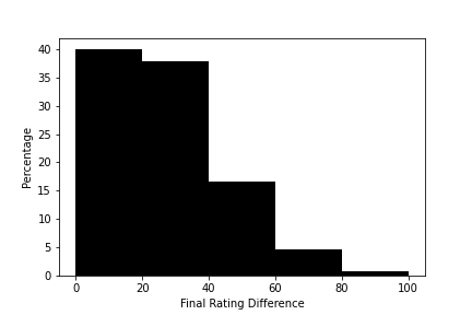
This is different from our simulation results because we're looking only at the final rating, not the maximum or minimum rating. We could compute the distribution of maximum fluctuation and compare to the simulated version, but they should end up looking roughly the same. From the probability distribution, we can calculate that, on average, we'll end up 22.7 rating points away from our initial rating, with a standard deviation of 17.6 rating points.

Reality check

While this is all interesting, it's based on a model of chess skill that doesn't necessarily reflect reality. People aren't probabilistic machines. They get tired and cranky. They get kicked out of games because of a faulty internet connection. They blunder their queen in a winning endgame, then tilt and lose 10 games in a row. A natural question, then, is how the ELO model holds up against the behaviour of real players.

For this purpose, I downloaded the ratings graph for 964 Lichess users over their last 100 blitz games. The player names came from the Lichess data dump, March 2024. Here's the distribution of their final ratings, relative to their initial ratings.

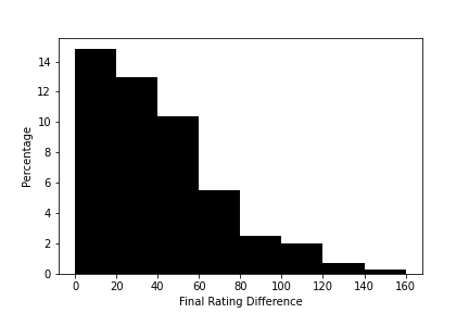
The shape of the distribution is similar to the one generated by the Markov model (see plot (d)), but in the real world, ratings seem to change a lot more. There are many plausible explanations for this:

• Players are not starting at their "true" rating, and could be recovering from an unlucky losing streak or coming off a lucky winning streak.
• The matchmaking isn't perfect and players can lose a lot of points to weaker players or win a lot of points from stronger players. Tournaments also match people of vastly different ratings.
• Someone's "true" playing strength can change even in a short period of time, e.g. they might learn a new opening trap that wins them a bunch of games.
• People don't play perfectly consistently.
• Lichess's Glicko-2 system might result in more ratings volatility (not sure on this one).

Here's the same plot for the max rating difference over all 100 games. For comparison, see plot (b).

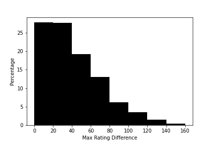
While it appears that some players are more stable than the ELO model predicted, with a max fluctuation of less than 20 points, this is deceptive. I didn't do a great job at cleaning the data, and the dataset includes friendly games that don't affect people's ratings, as well as games that were abandoned before they started. This flaw becomes more apparent in the cumulative distribution, which can be compared with plot (c).

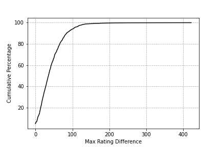
We see that a non-zero percentage of players stay at the same rating over all 100 games, which most likely means they exclusively play friendly games. I can think of two other factors that could make real-life ratings more stable than predicted by the ELO system:

• The simulations and Markov model don't account for draws. While draws aren't that common in blitz games between non-pro players, they still happen sometimes.
• They also don't account for the asymmetry of chess. Someone's effective strength can vary greatly depending on whether they're playing as white or black, and this could result in winning most of their games as white and losing most of their games as black.

Conclusions

I'm fed up with this investigation, so I'm not going to bother cleaning the data or doing any further analysis. In a future post, I do want to dig into the Lichess dataset and look at non-chess-related behaviours, like how often people ragequit.

What have we learned, then? Well, not much. The ELO rating system uses the sigmoid function to map rating differences to probabilities & expected score. Rating fluctuations within this system can be explored via simulation or Markov processes. And it seems reasonable to claim that players, whether they're probabilistic machines or real users on Lichess, mostly don't fluctuate by more than 100 rating points over 100 games, although this is entirely dependent on the person and the rating system under consideration.

The notebook containing all the analysis and plotting from this article can be found here

• Back to blog
• RSS feed

I'd be happy to hear from you at galligankevinp@gmail.com.