Board games and Markov chains

2022-08-28

Using Markov chains to model simple board games.

Tags: probability

Children of a certain age are drawn to mindless board games like Snakes & Ladders, which involve no skill or decision-making or social engineering or anything that a reasonable human might associate with the word "fun". The outcome is determined entirely by chance, in the form of dice rolls. The only pleasure I can imagine being derived from such games is the trickle of dopamine that comes from winning and the schadenfreude that comes from seeing a snake devour your opponent, which in my considered opinion is setting children up to become inveterate gamblers and psychopaths, respectively.

While that may be the case, there may be one redeeming aspect to these games, which is that they can be analysed using simple tools from probability. The state of the game, such as the position of the players, changes each round based on the output of a random number generator, such as a die 🎲. The next state depends only on the random output and the current state. This is a Markov process, and it can be analysed using nothing more than some matrix math!

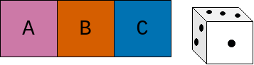
To illustrate what a Markov process (or Markov chain) is, let's consider a simple board game.

It has 3 squares: the start square A, the middle square B, and the end square C. Each turn, you roll a 6-sided die. If 1 comes up, you move back to A or stay on it if you're already there. If 2-5 come up, you advance to the next square. If 6 comes up, you go straight to C, no matter which square you're currently on. Once you're at C, the game is over and the state doesn't change anymore.

The states of the Markov chain that corresponds to this board game, and the probability of moving from one state to another (the transition probability), can be visualised as follows.

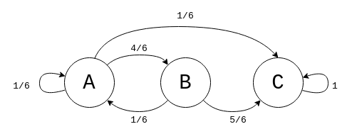
The circles are the states, which represent which square you're on. The arrows are labelled with the transition probability from one state to another. Based on the rules above, the transition probabilities for state A are: 1/6 to A, 4/6 to B, and 1/6 to C. They add up to 1/6 + 1/6 + 4/6 = 1, which makes sense because those are all the possible options and the probability of all possible options must be 1. From state B, there is a 1/6 chance of going back to A and a 5/6 chance of going to C, and 1/6 + 5/6 = 1. Finally, the probability of staying in C once you reach it is 1, because at that point the game is over.

The transition matrix $P$ expresses all of these probabilities at once:

$$P = \left[ {\begin{array}{ccc} p_{AA} & p_{BA} & p_{CA} \\ p_{AB} & p_{BB} & p_{CB} \\ p_{AC} & p_{BC} & p_{CC} \\ \end{array} } \right] = \left[ {\begin{array}{ccc} 1/6 & 1/6 & 0 \\ 4/6 & 0 & 0 \\ 1/6 & 5/6 & 1 \\ \end{array} } \right],$$

where $p_{ij}$ is the probability of going from state $i$ to state $j$. Each column in the transition matrix contains the transition probabilities for a state. The transition probabilites from A are in the first column, from B are in the second column, and from C are in the third column. Each row in the matrix contains the transition probabilities TO a state.

Let's say that $x^{(k)}$ is a vector containing the probabilities that you will be in state A, B or C after $k$ rounds of the game. Since we start off in state A with 100% probability,

$$x^{(0)} = \left[ {\begin{array}{c} p_A^{(0)} \\ p_B^{(0)} \\ p_C^{(0)} \\ \end{array} } \right] = \left[ {\begin{array}{c} 1 \\ 0 \\ 0 \end{array} } \right],$$

where $p_i^{(k)}$ is the probability of being in state $i$ after $k$ rounds. To get the probabilities for the $k$-th round, multiply the transition matrix by the probabilities for the $(k-1)$-th round:

$$x^{(k)} = P x^{(k-1)} = P P x^{(k-2)} = ... = P^{k} x^{(0)}$$

for $k>0$. So there is a fixed probability of being in any state after $k$ rounds of the game, which is determined entirely by matrix multiplication. Why does multiplying by the transition matrix give us the probabilities for the next round? If you multiply it out, you'll see that

$$x^{(k)} = P x^{(k-1)} = \left[ {\begin{array}{c} p_A^{(k-1)}p_{AA} + p_B^{(k-1)}p_{BA} + p_C^{(k-1)}p_{CA} \\ p_A^{(k-1)}p_{AB} + p_B^{(k-1)}p_{BB} + p_C^{(k-1)}p_{CB} \\ p_A^{(k-1)}p_{AC} + p_B^{(k-1)}p_{BC} + p_C^{(k-1)}p_{CC} \\ \end{array} } \right].$$

The probability of being in state A in the $k$-th round is the probability that we were in state A in the $(k-1)$-th round and stayed in A, plus the probability that we were in state B and transitioned to A, plus the probability that were were in state C and transitioned to A. The same applies to the other states. It alllllll makes sense when you multiply it out.

With these newfound powers, we can plot the probability distribution of being in any of the states on a given turn.

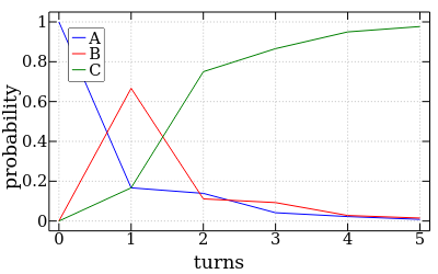
The probability of being in the end state, C, very quickly converges to 1. It's a short game. But how many turns should we expect it to take for the game to end? Will the game be over in time for tea, or will we be driven to blow our brains out by the pointless monotony of it all? This can be resolved using... linear algebra¹!

First, let $S_a=\{i:p_{ii}=1\}$ be the set of absorbing states, which are the states we can't escape from once we've entered them. In the case of our example game, $S_a = \{C\}$. Also let $\Chi$ be the set of all states and let $S= \Chi - S_a$ be the set of non-absorbing states.

Now let $\mu_i$ denote the expected number of turns to finish the game once we've reached state $i$. $\mu_i=0$ for absorbing states $i \in S_a$, because the game is already finished and there are no more turns left! For $i \in S$, $\mu_i$ is 1 (the next turn) plus the expected number of turns from the state we end up in after the next turn. When weighed by the probability of going to each state, this can be expressed as

$$\mu_i = \sum_j (1+\mu_j) p_{ij} = \sum_j p_{ij} + \sum_j \mu_j p_{ij} = 1 + \sum_j \mu_j p_{ij}.$$

We've already said that $\mu_i=0$ for absorbing states, so this can be rearranged as:

$$\mu_i(p_{ii} - 1) + \sum_{j\in S \backslash i} \mu_j p_{ij} = -1.$$

What this gives us is one linear equation and one unknown $\mu_i$ for each of the $k$ non-absorbing states. And we can solve the equations to find the average number of turns that the game will last!

To write the equations in matrix form, let $P_S = [p_{ij} : i\in S,j\in S]$. Basically, $P_S$ is the $k \times k$ submatrix of $P$ where we've removed all the rows and columns that correspond to absorbing states. And now our system of equations can be represented as

$$(P_S^T - I)[\mu_i : i \in S] = [-1],$$

where $I$ is the identity matrix, $[\mu_i : i \in S]$ is the column vector of unknowns, and $[-1]$ is a column vector of $k$ -1s.

I have probably committed an atrocity of math notation there, but anyway. Solving this system of equations for our example game gives $\mu_A=2.3$ and $\mu_B=1.39$. Homework for the reader: verify this result by hand or by plugging the equations into a linear algebra solver of your choice. Or, grab a die, play the game a bunch of times, track how many turns each game takes, and average them afterwards to get an estimate.

The techniques I've covered here also apply to Snakes & Ladders, Monopoly (which are the best properties to buy?), the number of times you need to flip a coin before getting 5 heads in a row, and any other situation that can be modelled as a Markov process!

Appendix: The Code

The supporting code for this article is available as a GitHub gist. I wrote it in the J programming language, which is (in)famous for looking like gobbledygook if you're not familiar with it. I was originally planning to walk through the code line by line, but I will instead write about J another time.

• Back to blog
• RSS feed

I'd be happy to hear from you at galligankevinp@gmail.com.